kscottz

Fish Eye Lens Dewarping and Panorama Stiching

The entire panorama stitching process as one big image.

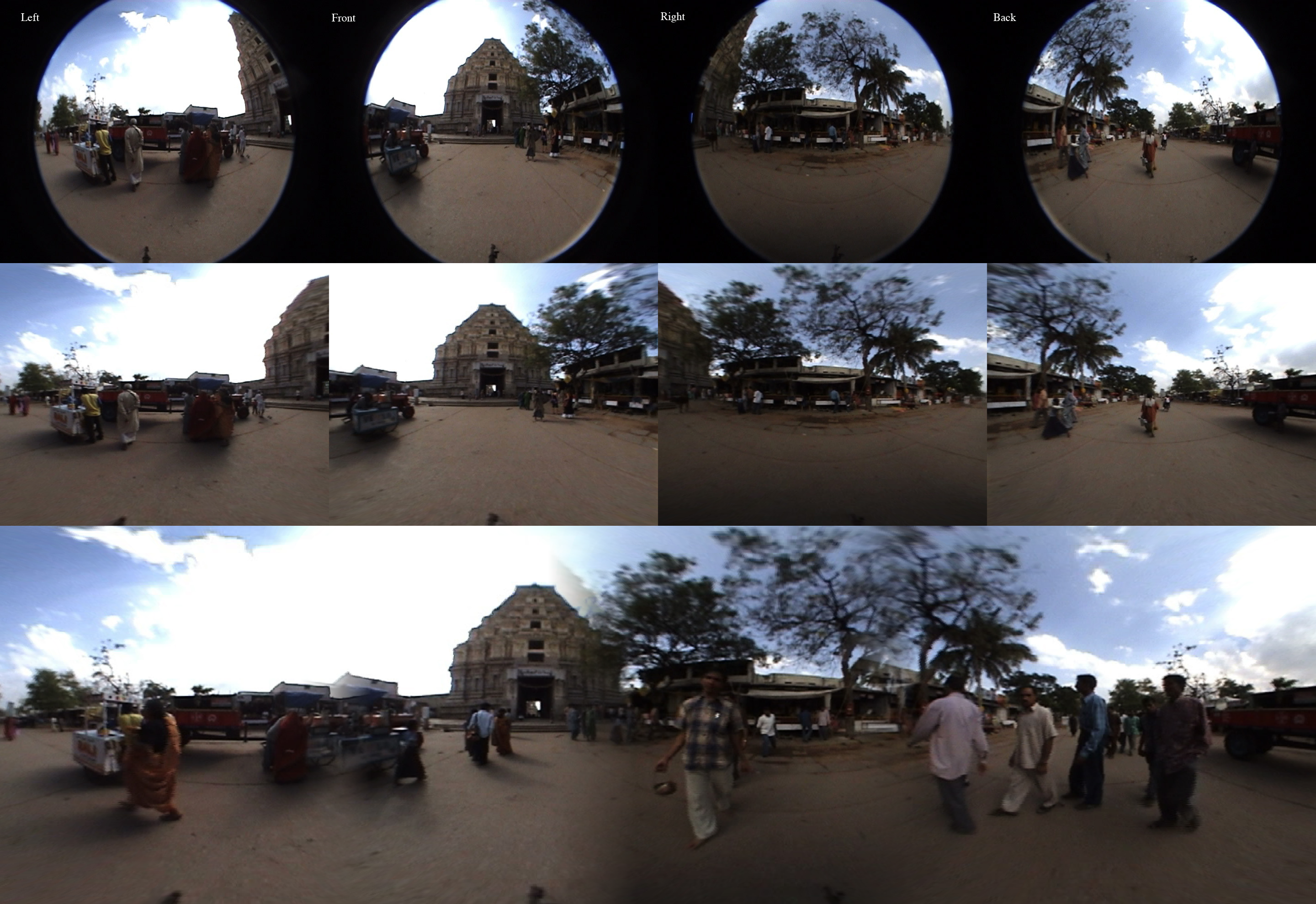
The entire process as one big image.

I was challenged to see if I could create 360 degree view panoramas from a series of fish eye images taken at right angles to one another working from this tutorial. I modified the code from my 360 lens dewarping project to create the code for this project which you can check out here. There are roughly two types of fisheye images, circular fisheye lens that map a sphere onto the image plane, and full frame fisheye lens that map the input image to the entire rectangular image plane. The data I was working with was from a circular fisheye, which is significantly easier to reason about.

There are a couple of different ways you can approach the problem of fisheye lens dewarping. The first, and probably more robust approach is to develop a camera lens model that accurately represents the fish eye lens distortion, and apply that lens dewarping to the image. In the absence of a calibration data, particularly for full frame fisheye’s, you would then need to manually tune the camera model parameters to dewarp the image, or use some of the image data to get a back of the envelope approximation of the camera parameters. The second, and in my opinion the easier, albeit slightly less robust approach, is to create a mapping from the output image pixels in terms of phi and theta in a circular coordinate system, and map that to pixels in the input image. The basic idea is that in the output image each pixel represents some steradian on the input image. The best way to think about a steradian is as a “pixel” on the sphere, or the square mapped out by latitude and longitude lines. Each steradian then maps to a point on the image plane, which you can calculate by doing a spherical to Cartesian conversion and dropping the value that is in the normal to the image plane.

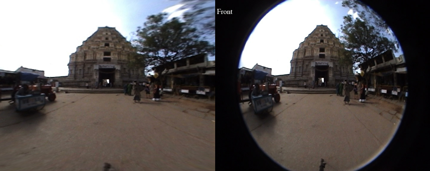
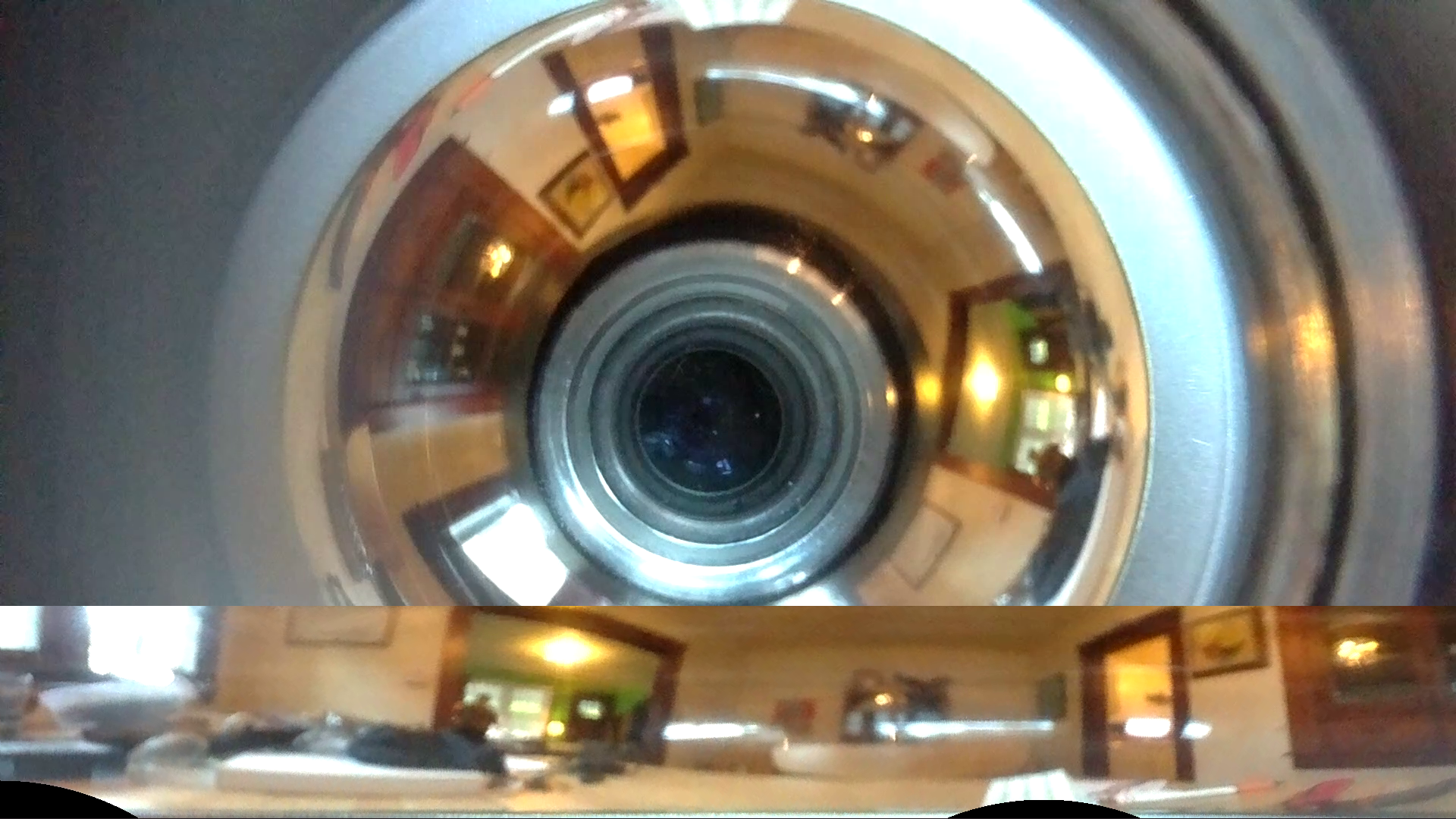
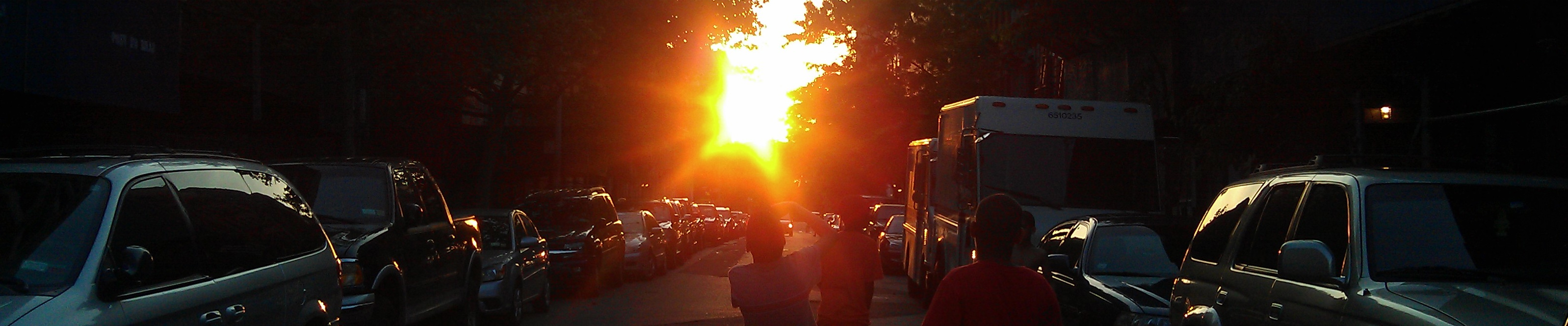
Dewarped image on the left and input circular fisheye image on the right.

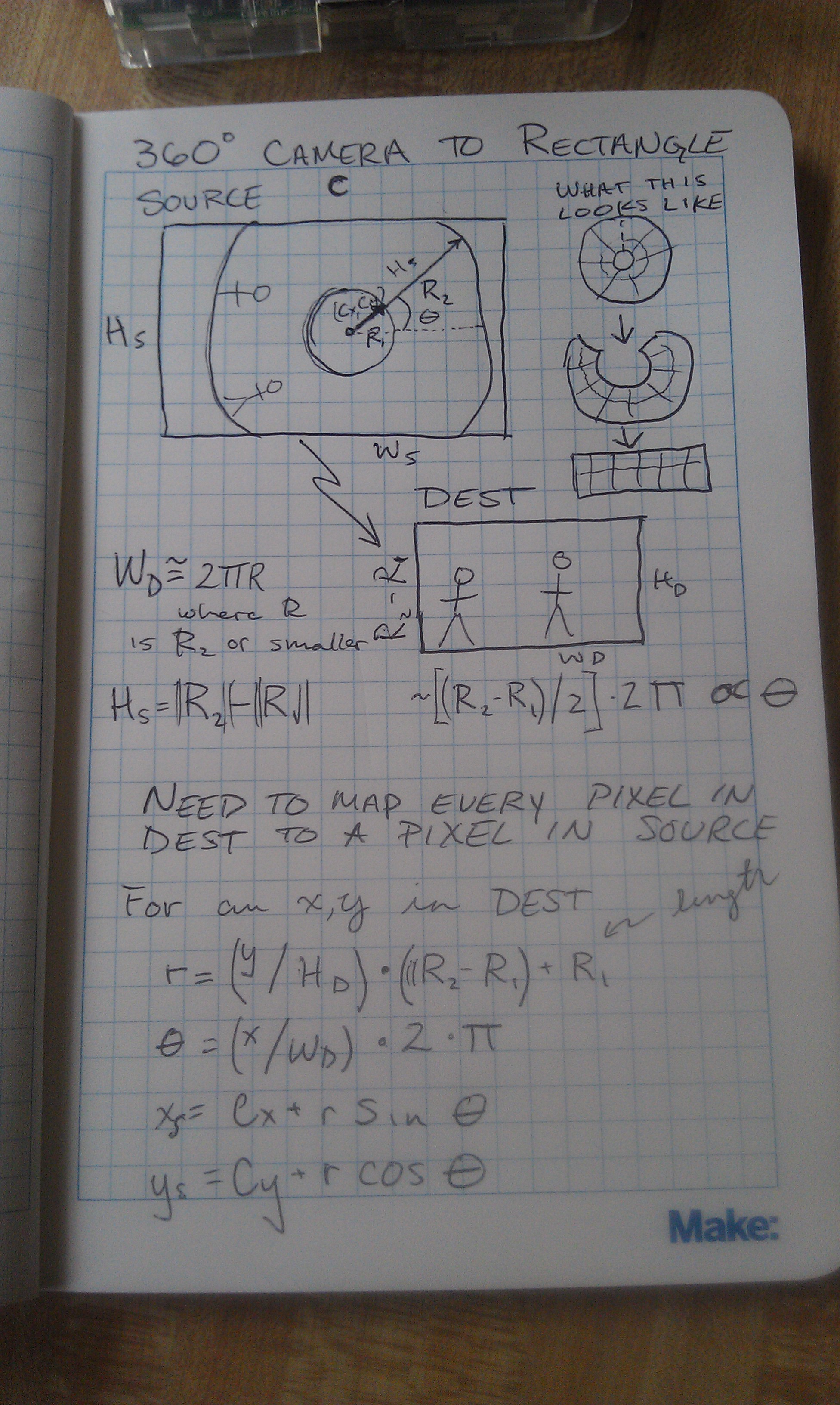
For example, in my code, I first create an output image and assume each x and y position on the image maps to somewhere roughly between 0 and 180 degrees (0,pi) for both phi and theta. In my model the direction pointing straight out of the camera is called y, so I then do a spherical to Cartesian conversion assuming a unit sphere. Since the unit sphere is at the origin, I shift the sphere and rescale it to be of unit length, and then multiply the result by the input image dimensions. An easier way to think of it is this:

Destination image pixel (X,Y) –> scale to unit length –> convert to between zero and pi –> do spherical to Cartesian conversion –> rescale to get values between 0 and 1 –> multiply by the input image dimensions to get input pixel (X,Y).

The map is a bit tedious to create, but once you have it, OpenCV can really quickly push pixels around and give you a result.

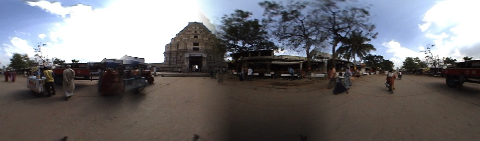
Panorama dewarped from four fish eye images.

The next step was to do the panorama stitching. To do this I first matched ORB keypoint between two successive pairs of images. Since I knew the images were vertically aligned, all I needed to calculate was the x value that is the horizontal offset. To do this I used the median x difference between the two sets of points (the median in this case acts as a poor man’s RANSAC to remove outlier matches). I then used this x offset to construct an alpha mask that I could use to smoothly blur the two images together. I played with this for a little while and I found a nonlinear mapping seemed to work a lot better. There are some problems with the images as they don’t seem to be taken at the exact same time, but for a half a day’s worth of work I am very pleased with the results.

Dewarped Panoramic Images From A RaspberryPi Camera Module

I got back from my cross country trip and in my mail box was a brand new RaspberryPi camera module from Element14. I needed a chill night at home so I setup the camera module and decided to see what I could do with it. After upgrading my pi to the latest version of wheezy and doing the requisite setup for the camera and the wireless card I was getting images. The setup for the camera module is fairly easy and wheezy has a few really nice command line programs for capturing, compressing, and delivering images to a remote host. The RPI foundation has a nice tutorial here. I am *extremely* impressed with the quality of the RPI camera module, the image quality far exceeds that of the built-in cameras on my macbook air and my lenovo laptop. At full resolution the camera module’s image quality is akin to a point and shoot camera from a few years ago. Not a bad feat for $20.

I wanted to do some interesting processing from the camera images. Given the performance of the pi using python I opted to look for an approach where I would use the pi as a dumb ip camera and process the images on the remote host. I remembered that I had a Kogeto 360 degree camera for iPhone in my basement. I don’t have or want iPhone so the lens was useless to me as is. After some careful twisting and prying I was able to remove the lens from the mount. I decided to whip up a quick adapter using just some silly putty and cardboard.

Parts for my hacked camera shim.

Since my RPI camera module is just loose, and not mounted to anything, I needed a non-destructive and quick way to attach the lens to the camera. I created three cardboard shims using my pocket knife, one that fit snugly to the camera, one that fit snugly to the protrusion on the lens, and one to space the two parts out. I used silly putty to “glue” the boards together while allowing me to slide them around to get the alignment just right. Silly putty works great for this as it is non-conductive and easy to pick out the RPI camera board without breaking it. Also cleans up fairly easily. After a little of trial and error I got a working prototype.

The final assembled lens shim. Hopefully I can CAD up a permanent one and 3D print it soon.

I switched on the raspberry pi and started getting images. The 360 degree camera doesn’t use the full image frame. Instead it projects a donut onto the image plane that we can dewarp to get a full panoramic image. The image below shows most of an input image with the dewarped result overlaid.

The input image with the dewarped image over laid at the bottom.

You can see that input image has a basically a “doughnut” where the actual image appears, the rest is just noise. You can see a minute of raw camera video here to get a better sense of what I mean. The trick to do the dewarping is to take that doughnut, put a slice in it, and uncurl it to a rectangle that looks like a normal image. To do this you need to figure out a couple things, the center of the doughnut, the radius of the “doughnut hole”, and the outer doughnut radius. Once you have this stuff the mapping for the camera is basically translating every point in the destination image to a point in the source image using a radial (r,theta) representation. I posted the notes from my notebook to give you a better idea of what I did.

$Doing the doughnut mapping from the destination image to the source image.$

Doing the doughnut mapping from the destination image to the source image.

I coded this all up in python using the cv2.remap function. For this function you just create a list of every pixel in your destination image and tell it where to point to in the source image. It takes awhile to create the map because I used naive python looping, but once the map is created the mapping can be done in nearly real time. I tossed the code into this github repo. It took me a bit of time to figure out that mapping was from destination to source versus the other way around. I am also still having some problems with encoding the output video so I just dumped them to file and had ffmpeg stitch them back together into a video. Here is my first draft of the code (a bit of a hack).

I used a quick command line ffmpeg call to stitch the still frames I produced back into a video so I could post it YouTube. This is a really neat feature of ffmpeg that has saved me quite a few times. the raw command is (avconv -r 32 -f image2 -i ./FRAME%05d.png -b:v 1024K output.mpeg).

Hopefully when I get some time later next week I will modify this script to perform dewarping on live streams from the RaspberryPi. I also would like to fab a legitimate adapter using a 3D printer. If I manage to get that done I will toss the design files in the github repo and thingaverse.

Solving Autostereograms AKA Magic Eyes

shark

This week I’ve been playing with autostereograms, also called magic eye images. MagicEye images were big in the 90s when I was a kid/teen and every mall had a kiosk peddling framed copies. I wanted to see if I could reconstruct the depth map from the image using a little bit of image processing. Autostreograms work because your eye/brain is really into creating stereo depth maps, and if you set your eye’s focus at a point behind the image your brain basically goes a bit haywire and tries to build a depth map in the plane of the image. Getting your vergence point to sit behind the image plane requires some practice; so if at first you don’t see the image keep trying. I really recommend reading the wikipedia article linked to above as it is really well written with a lot of fantastic diagrams.

To do this project I created a small data set of “wall-eyed” random-dot autostereograms. There are other kinds of stereograms, that can be viewed in different ways, but I felt the random-dot ones would be slightly easier to decode. The basic premise is that for every small set of horizontal pixels there is a corresponding row of pixels some distance away. The distance between the matching rows segments is what your brain uses to get the depth map. The matching of the rows of pixels is periodic with a period related to the vergence distance you must view the image at. Figuring out the period of the image is easy, if you look at the image you can basically see columns of pixels. For most autostereograms there are usually between 6 and and 20 for a normal image, the horse image above has seven instances of the repeating patern. If you have an image that is 600 pixels wide, with about six columns, the pixel, or set of pixels at [0,0] will have a correspondence at roughly [100+d,0], where the value of d is the depth value.

I baked up a naive algorithm in about 90 minutes and had an early prototype. The basic idea is that you iterate over the rows in the image, and for a small chunk of pixels in that row (roughly ten pixels) you search a window around where the correspondence should exist, and then record that value in a depth map. So for our example image 600 pixels wide, you would try to match pixels [0:10,0] with [100:110,0], [101:111,0] and so on until you found a decent match. For my first example I used the gray scale sum of absolute pixel differences. You could do a correlation, but I thought that the simple solution should suffice. It is worth noting that you can also move up to frequency space and do a multiplication of the spectra but that seemed like a lot of work. I googled a bit and found this example that does just that. That solution seems to get stronger edges, and work on a few different kinds of stereograms, but I would argue mine gets betters depth maps.

My first pass, using naive python looping worked but it was as slow as molasses in January. I decided to see if I could speed things up. The first speed hack I tried was to use an integral image. An integral image is an image where each pixel is the sum of the pixels above and to its left. Integral images are great if you want to calculate lots of different average values across an image really fast, and they are what makes Haar Cascades and face detection possible. In an integral image, once the integral is computed, the sum, and average of any area in the image can be computed with in just four look-ups, and three additions, which is a decent time savings. I modified my code and got maybe a 10-20% speed up (I didn’t bench mark it). Since the operations are done row-wise and each row is independent of the next one this algorithm is really well suited to parallelization. I decided to try my hand at doing some image processing using the python multiprocessing library. It took me about an hour to chunk out the code and get everything running, but it did improve performance significantly (a little less than 4x). I need to go back and refactor the code to deal with some bounds issues, which is causing the horizontal lines in the image, and perhaps use shared memory, but the results are well worth the effort. You can take a look at the code for yourself at this repo, I’ve put a gist of the code below for reference.

If I get some more time I want to see how much of a speed up Numba can get the naive implementation and possibly do some bench marking of the different approaches. I also need to remove the banding caused by the multiprocess “chunking.” The algorithms performance seems to be very dependent on the search window size so I would like to find a more robust way of determining the size of the search window, possibly by looking at low end of the FFT spectrum.

PyCon Talk and Tutorial

I wanted to put all of my PyCon stuff in one place for easy reference. When I get a moment to breathe I want to do a write up about what it took to put everything together.

Here is the short talk I gave.