I got back from my cross country trip and in my mail box was a brand new RaspberryPi camera module from Element14. I needed a chill night at home so I setup the camera module and decided to see what I could do with it. After upgrading my pi to the latest version of wheezy and doing the requisite setup for the camera and the wireless card I was getting images. The setup for the camera module is fairly easy and wheezy has a few really nice command line programs for capturing, compressing, and delivering images to a remote host. The RPI foundation has a nice tutorial here. I am *extremely* impressed with the quality of the RPI camera module, the image quality far exceeds that of the built-in cameras on my macbook air and my lenovo laptop. At full resolution the camera module’s image quality is akin to a point and shoot camera from a few years ago. Not a bad feat for $20.
I wanted to do some interesting processing from the camera images. Given the performance of the pi using python I opted to look for an approach where I would use the pi as a dumb ip camera and process the images on the remote host. I remembered that I had a Kogeto 360 degree camera for iPhone in my basement. I don’t have or want iPhone so the lens was useless to me as is. After some careful twisting and prying I was able to remove the lens from the mount. I decided to whip up a quick adapter using just some silly putty and cardboard.
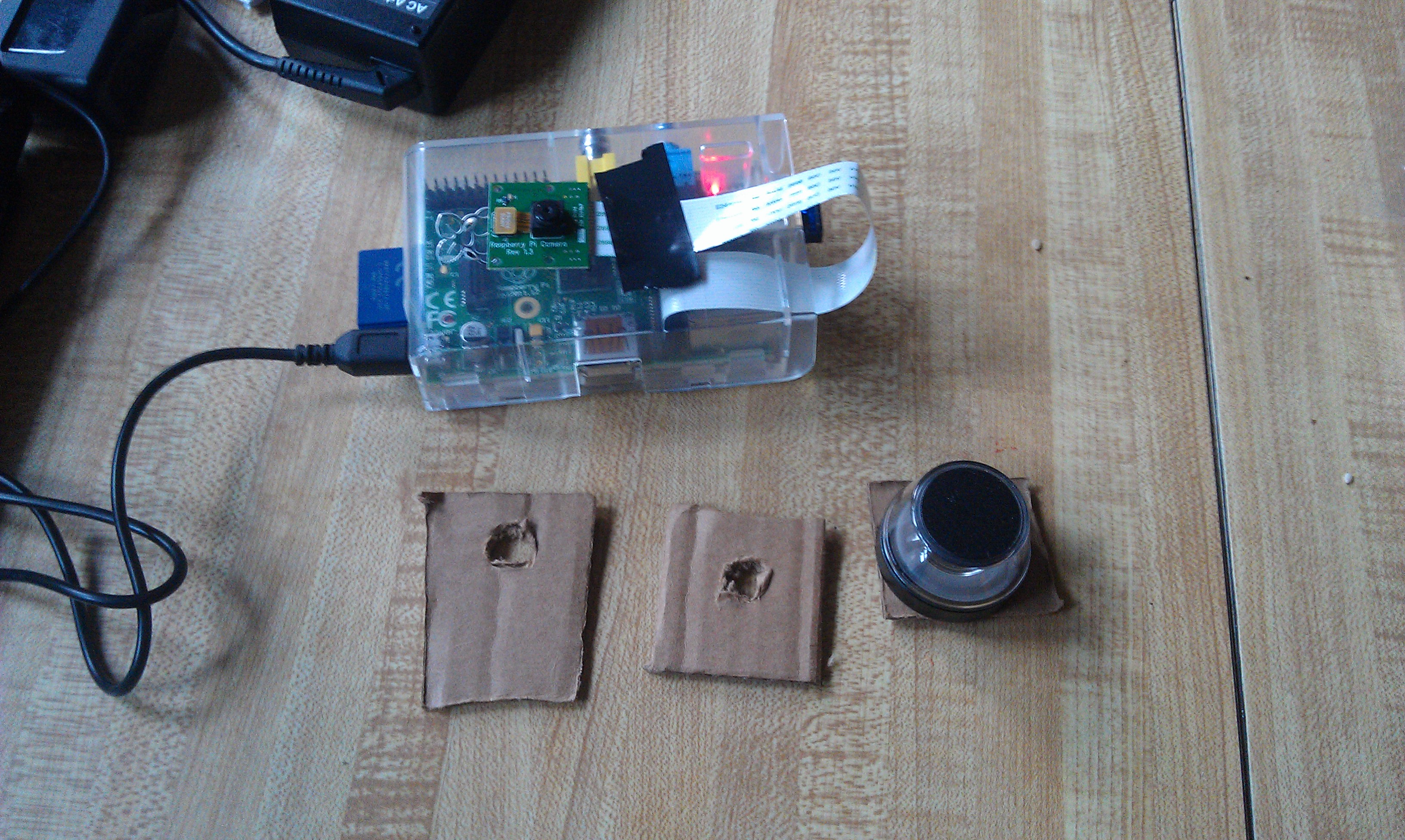
Parts for my hacked camera shim.
Since my RPI camera module is just loose, and not mounted to anything, I needed a non-destructive and quick way to attach the lens to the camera. I created three cardboard shims using my pocket knife, one that fit snugly to the camera, one that fit snugly to the protrusion on the lens, and one to space the two parts out. I used silly putty to “glue” the boards together while allowing me to slide them around to get the alignment just right. Silly putty works great for this as it is non-conductive and easy to pick out the RPI camera board without breaking it. Also cleans up fairly easily. After a little of trial and error I got a working prototype.
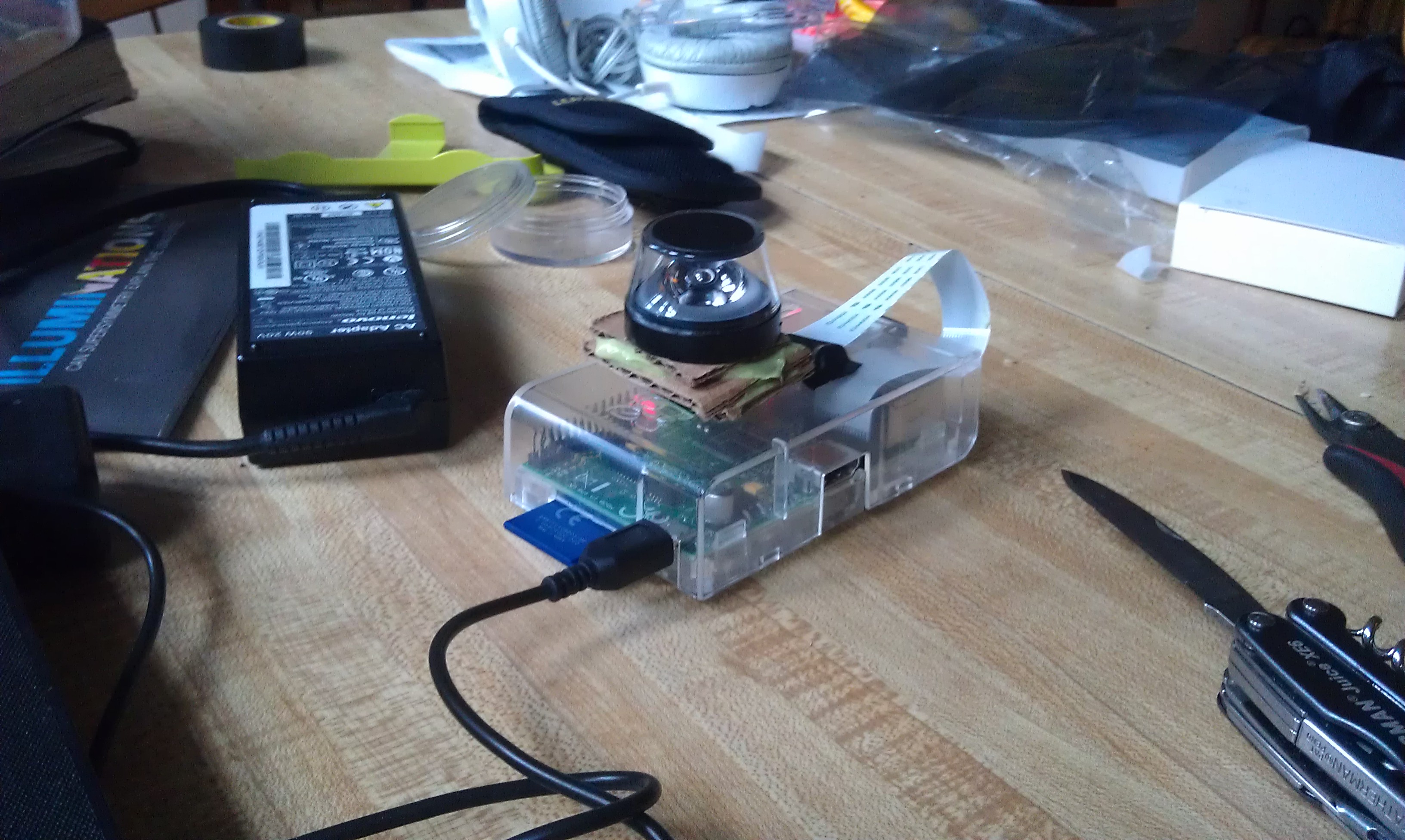
The final assembled lens shim. Hopefully I can CAD up a permanent one and 3D print it soon.
I switched on the raspberry pi and started getting images. The 360 degree camera doesn’t use the full image frame. Instead it projects a donut onto the image plane that we can dewarp to get a full panoramic image. The image below shows most of an input image with the dewarped result overlaid.
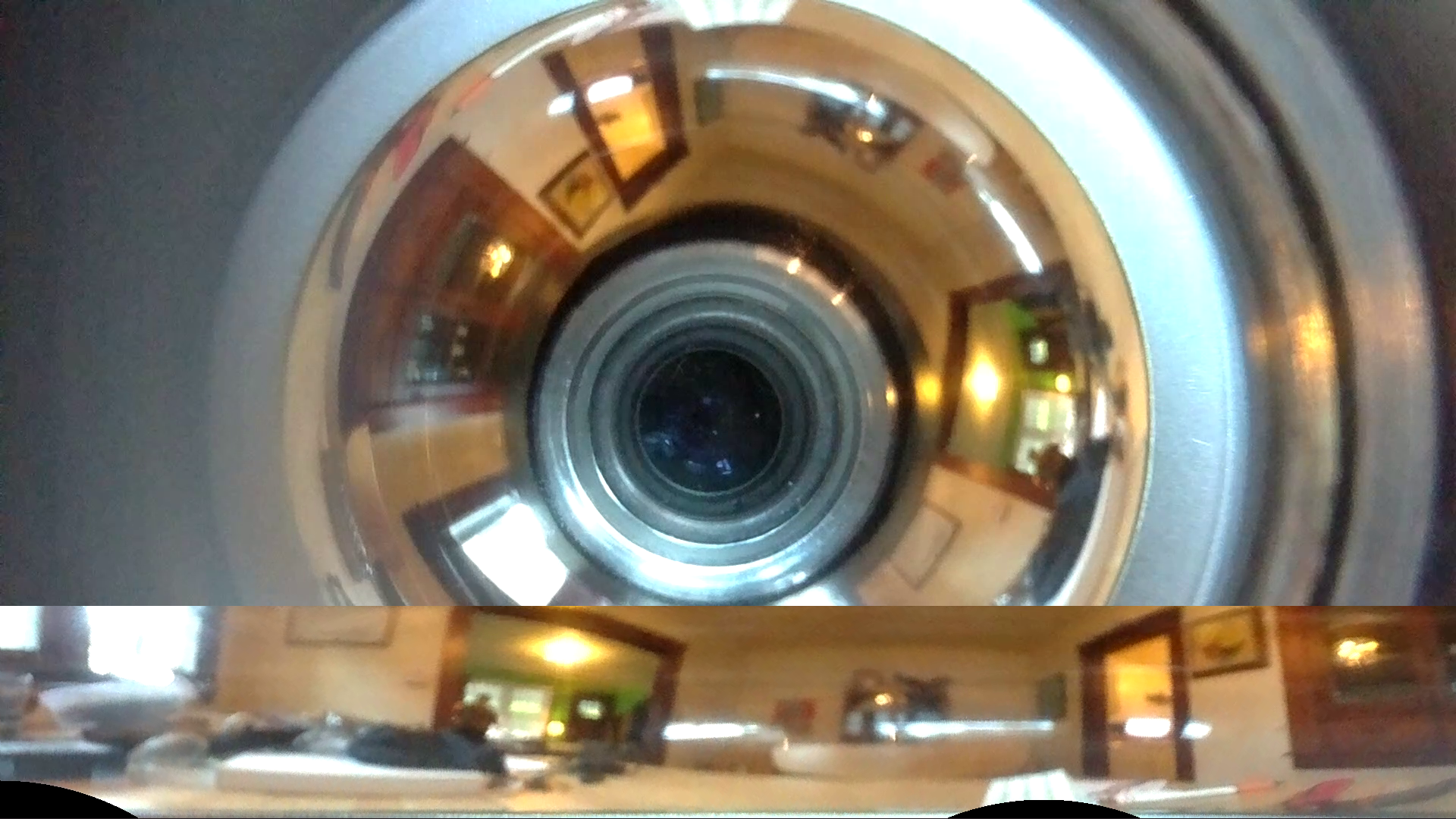
The input image with the dewarped image over laid at the bottom.
You can see that input image has a basically a “doughnut” where the actual image appears, the rest is just noise. You can see a minute of raw camera video here to get a better sense of what I mean. The trick to do the dewarping is to take that doughnut, put a slice in it, and uncurl it to a rectangle that looks like a normal image. To do this you need to figure out a couple things, the center of the doughnut, the radius of the “doughnut hole”, and the outer doughnut radius. Once you have this stuff the mapping for the camera is basically translating every point in the destination image to a point in the source image using a radial (r,theta) representation. I posted the notes from my notebook to give you a better idea of what I did.
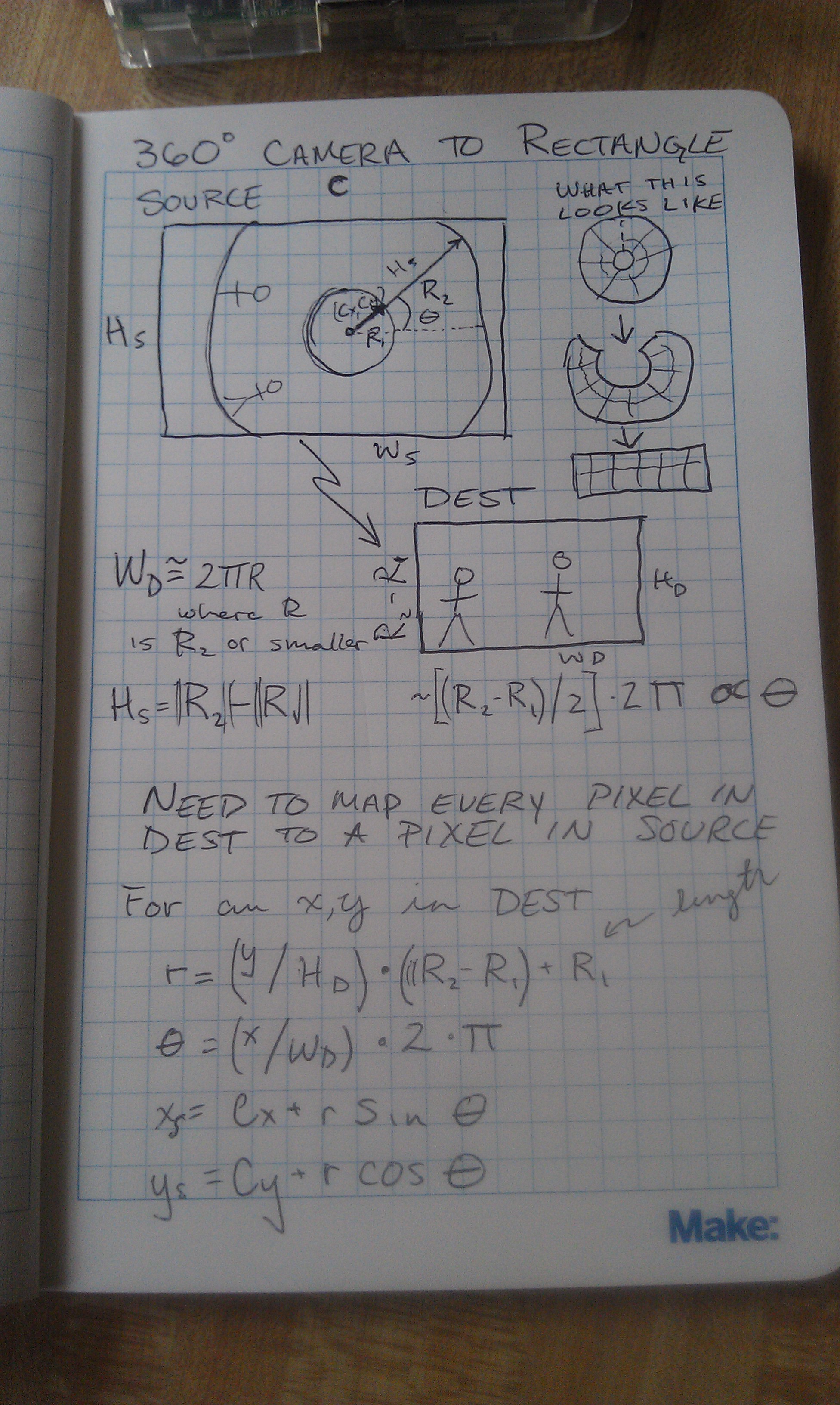
Doing the doughnut mapping from the destination image to the source image.
I coded this all up in python using the cv2.remap function. For this function you just create a list of every pixel in your destination image and tell it where to point to in the source image. It takes awhile to create the map because I used naive python looping, but once the map is created the mapping can be done in nearly real time. I tossed the code into this github repo. It took me a bit of time to figure out that mapping was from destination to source versus the other way around. I am also still having some problems with encoding the output video so I just dumped them to file and had ffmpeg stitch them back together into a video. Here is my first draft of the code (a bit of a hack).
I used a quick command line ffmpeg call to stitch the still frames I produced back into a video so I could post it YouTube. This is a really neat feature of ffmpeg that has saved me quite a few times. the raw command is (avconv -r 32 -f image2 -i ./FRAME%05d.png -b:v 1024K output.mpeg).
Hopefully when I get some time later next week I will modify this script to perform dewarping on live streams from the RaspberryPi. I also would like to fab a legitimate adapter using a 3D printer. If I manage to get that done I will toss the design files in the github repo and thingaverse.