kscottz

Open Skinner Box – PyCon 2014

I’ve been hacking like a fiend on nights and weekends for the past few months trying to get ready for PyCon. This year I wanted to do an introductory talk about how you make internet enabled hardware using Python. The first step of this process is figuring out what hardware you want to make. I decided I wanted to do something for my pets as I am splitting my time between Boston and San Francisco and I can be gone for a week at a stretch. My friend Sophi gave a great talk at last years Open Hardware Summit about creating a low-cost nose poke detector for research and I decided I could sorta do a riff (in the jazz sense) on that idea. I decided to create an Open Skinner Box using a RaspberryPi and a few parts I had around the house.

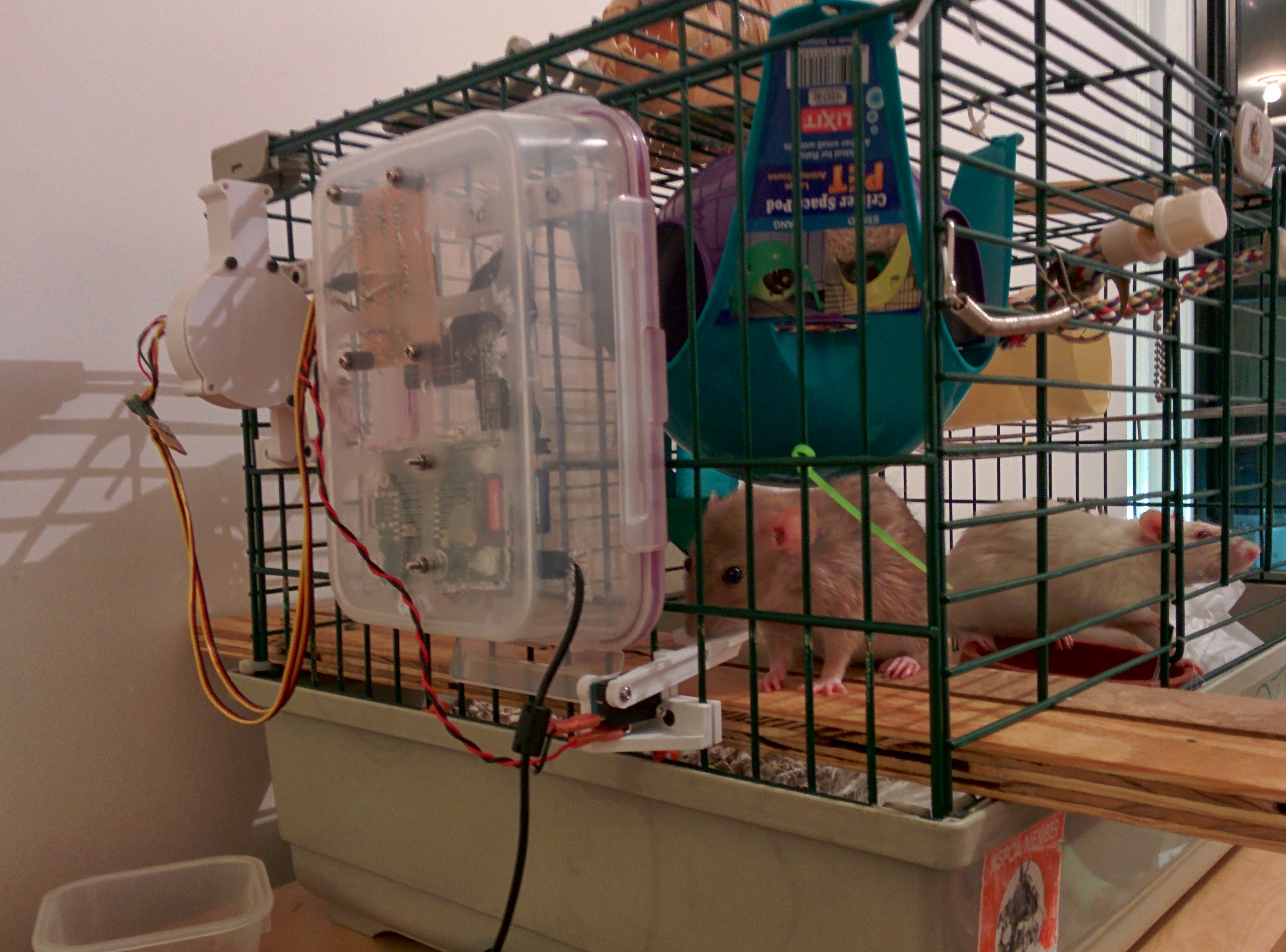
Open Skinner Box in situ

A Skinner Box, also called an operant conditioning chamber, is a training mechanism for animal behavior. Generally a Skinner box is used to create some behavior “primitives” that can then be stringed together to do real behavioral science. The most basic Skinner Box has a cue signal for the animal (usually a light or buzzer), a way for the animal to respond to the cue (usually a nose poke detector or by pressing a lever), and a way to reward the animal usually using food. The general procedure is that the animal hear’s or sees the cue signal, performs a task, like pressing the button, and then gets a treat. This is not too far off with the training most people do with their pets already. For example, I have the rats trained to come and sit on my lap whenever they hear me shake a container with treats.

The cool thing about a Skinner box is that they are used to do real science. As a toy example, let’s say you wanted to test if some drug may have an adverse effect on learning. To test this scientifically you could have two groups of rats, one set of rats would get the drug and the others wouldn’t. We would then record how long it took the rats to learn how to use the Skinner box reliably. The scientist doing the experiment could then use this data to quantify if the drug has an effect and if that effect scales with the dosage of the drug.

So what does it do?

I wanted to create not just a Skinner Box but a web enabled Skinner Box, a sorta internet of things Skinner Box. So what features should it have? I came up with the following list:

I should be able to see the rats using the Raspberry Pi’s camera.
The camera data should be used to create a rough correlate of the rat’s activity.
The box should run experiments automatically.
I should be able to buzz and feed the rats remotely.
The web interface should give a live feed of all of the events as they happen.
The web interface should be able to give me daily digests of the rats activity and training.

The Mechanical Bits

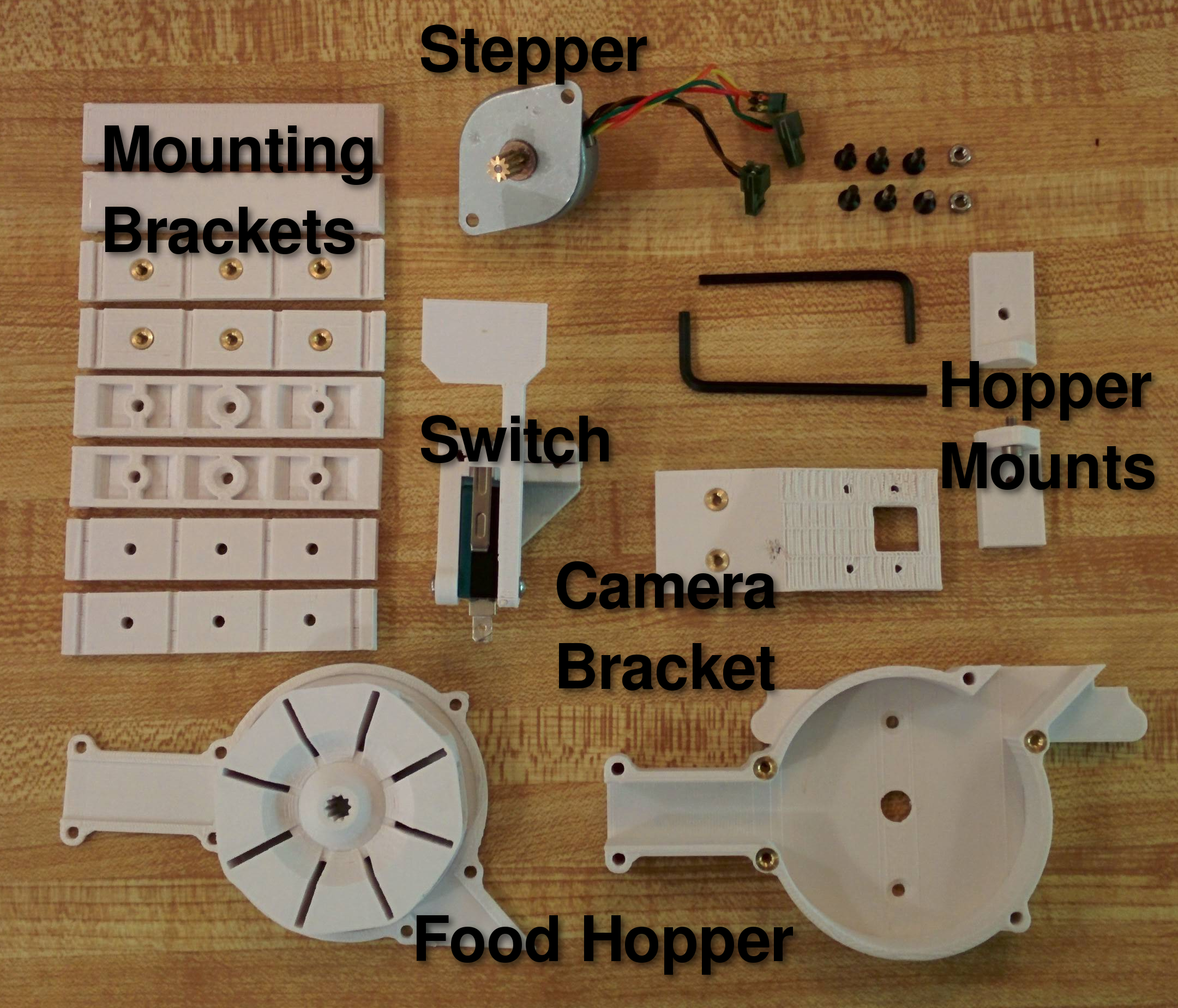
Mechanical Bits of the Open Skinner Box

To build the Skinner Box I got some help from a mechanical engineer friend of mine. He is a 3D printing whiz and designed the mounting brackets, food hopper, and switch mechanism for the Skinner Box. One of the cool things I learned in this process was how to use threaded brass inserts for mounting the parts to the cage and attaching the different parts to one another. There is a great tutorial here as well as this video. The source files for all the parts are now up on thing-a-verse if you would like to build them.

The Electrical Bits

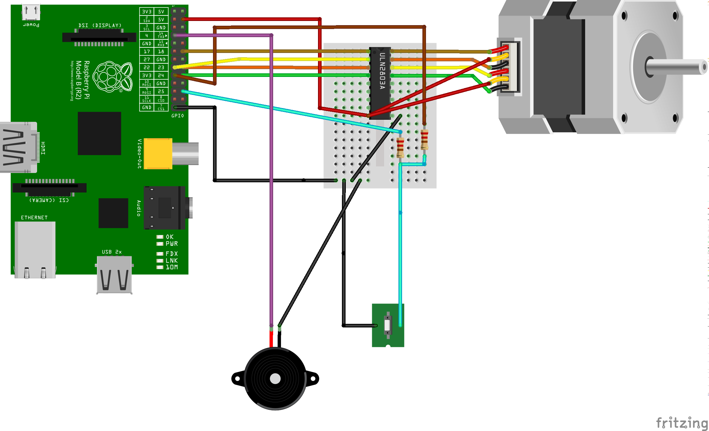
Skinner Box schematic – originals are in the github repo for the project.

For the electrical components in the project I used the Raspberry Pi’s GPIO pins to control the stepper, read the switch, and run the buzzer (although one could easily use the audio out). I opted to run the stepper using the RaspberryPi’s 5V source and it seems to have just enough juice to run the stepper motor. The stepper is controlled via four GPIO pins (two for each coil). The GPIO pins and the 5V source are connected to a LN2803 Darlington array that shunts the 5V source to the stepper based on whether the GPIO pins. In the next revision I will probably use a separate stepper driver and a beefier stepper like a NEMA 17. I soldered everything to a bread board for this revision but I will probably get PCBs fabricated for the next revision. When I was soldering and debugging the board I found ipython super useful. I could send each of the GPIO pins high or low and then trace the path with my multimeter. I have put both the Fritzing CAD files and a half-complete bill of materials up on github if you would like to replicate my work.

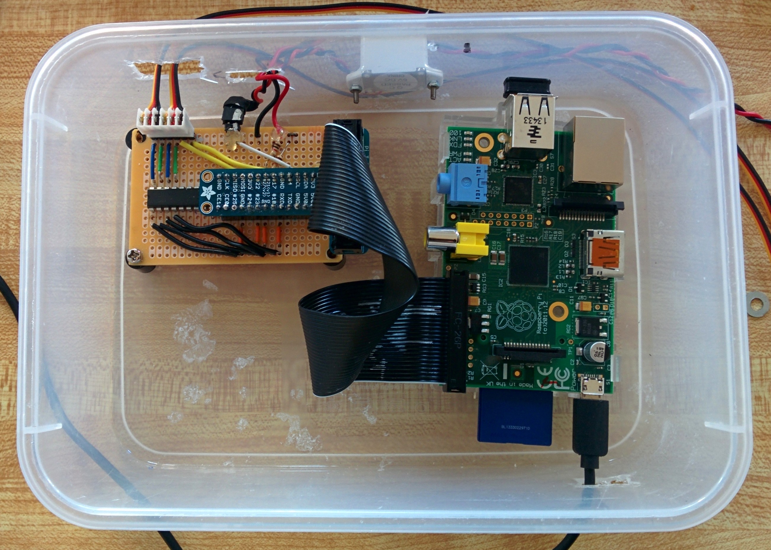
Finished Open Skinner Box electrical components.

The Software Bits

Because I was presenting this project as an intro lesson PyCon I wanted to use as many python libraries as possible. Right before the conference I open-sourced all of the code and put it in this github repository. Some of the components I used, for example matplotlib, are sub-optimal for the task but they get the point across and minimized the amount of java script I had to write. The entire app runs in a bottle web server with the addition of greenlets to do some of the websocket work. I set the webserver up to use Bootstrap 2.3.2 to make everything look pretty. For data persistence I used MongoDB. While you can get Mongo to build and run on a RaspberryPi in retrospect I really should have dug into the deep storage of my brain and used something like PostgreSQL. Mongo is still too unstable, and difficult to install on the Pi.

The general theory of operation is that there is the main web server that holds four modules, three of which are wrapped in a python thread class. These modules are as follows:

Hardware Interface – uses GPIO to buzz the buzzer, monitor the switch, and run the stepper.
Camera Interface – uses OpenCV, PiCamera, and Numpy to grab from the camera, save the images, and monitor the activity.
Experiment Runner – looks at the current time and decides when to begin and end experiments (e.g. it rings the buzzer, waits for the rat to press the lever, and dispenses a treat.
Data Interface – Stores event,time stamp pairs to Mongo, does queries, and renders matplotlib graphics

To get all of the modules to communicate cleanly I used a simple callback structure for each module. That is to say each module holds a list of functions for particular events, and when that event happens the module iterates through the list and calls each function. For example, whenever there is a button press the button press loop calls the callback function for the data interface to write the event to the database, a second callback tells the experiment runner that the rat pushed the lever, and a third callback renders the data to the live-feed websocket.

Rat Stats — need to replace this with some Javascript rendering.

All routes on the webserver basically point to one or more of the modules to perform a task and create some amount of data to be rendered in the bottle template engine. For example for activity monitor page I have the DataInterface module query Mongo for every activity event in the past 24 hours and I then render it using matplotlib and save the result to a static image file. The web server then renders the template using the recently updated static image file. While this works, matplotlib is painfully slow. To control the feeder and buzzer remotely I simply have post events that call the dispense and buzz methods on the hardware interface. The caveat here is that these methods are non-block and are guarded simply by a flag. So for example, if you hit the feed button multiple times in a row really fast only the first press has an effect.

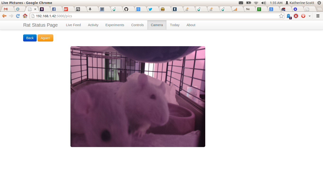
Skinner Box Live Shot

The camera module seems to work reasonably well for this project and I amazed by the image quality. The only drawback with the camera module is that basically you have to choose between still images and a stream of video data right now there is now really good way to both debuffer the camera stream and process the individual frames. I opted to take the less complex route of just firing the camera for still frames at the fasted rate it would support which is about once a second. Because of processing limitations on the pi I need to scale the image down to about 600×800 to do my motion calculation. For the motion calculation I just perform a running frame difference versus a more computationally costly optical flow calculation. This is a reasonably good approximation of net motion but it is subject to a lot of spikes when the lighting changes (e.g. when you turn the lights for the room on). Additionally in my haste of getting this project up and running I opted not to put a thread lock around the camera write operation. This means that sometimes when you visit the live image page you get a half finished frame. This is something that I will address soon.

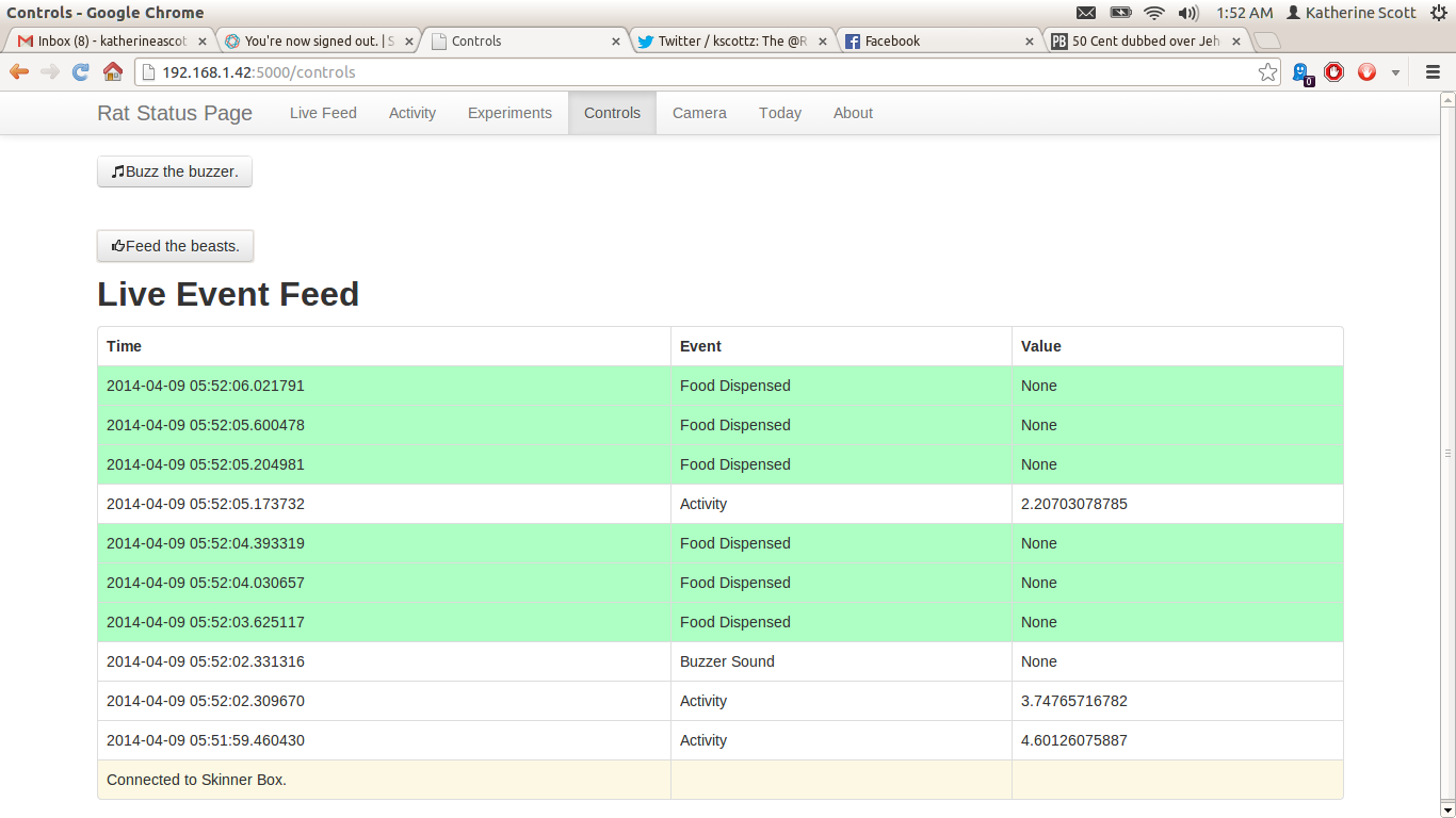
Live Events Feed

Putting it all together.

I have tested the system on the rats with some limited success (see the videos below). There are some kinks I still need to work out that prevent me from running the system full time. For example, the current food hopper wheel jams fairly frequently and so farm seems to only deliver food 2-3 times before jamming. Also the buzzer I used is exceptionally annoying, and since the rats live in my bedroom I don’t want to run protocols at night when the rats are most active(rats a nocturnal). Moreover, I don’t think my current pair or rats is suitable for training. I have one exceptionally old rat (almost three to be exact); and while she is interested she lacks the mobility to perform the task. The other rat has been one of the more difficult rats I have tried to train. Normal rats can learn to come when called (or when I shake the treat jar) this rat is either too timid or too ambivalent to care most of the time.

Building a Better Mouse Trap

The Skinner box runs reasonably well at the moment but there are quite a few things I would like to do to make it more user friendly and robust. Ultimately I would like to harden the designs and then turn them over to someone to commercialize. As with an engineering task design is a process, and you get a kernel of working code and then improve and build upon it until you finally reach a working solution. Here is what I would like to do in the next revision:

Replace Mongo with Postgre SQL.
Replace Matplotlib with a javascript rendering framework
Fix the camera thread lock issue and create a live stream of video and also store images to the database.
Move the food hopper to an auger based design to minimize jamming.
Add a line break sensor to make sure the rats get fed from the food hopper.
Add an IR LED illumination system for the camera and add a signal LED to work with the buzzer.
Improve some of the chart rendering to support arbitrary queries (e.g. how well the rats did last week over this week.
A scripting language for the experiment runner. Right now the experiment runner buzzes and waits for a button press, but really I think the rats should start with random food deliveries and work up to the button press task.

Fish Eye Lens Dewarping and Panorama Stiching

The entire panorama stitching process as one big image.

The entire process as one big image.

I was challenged to see if I could create 360 degree view panoramas from a series of fish eye images taken at right angles to one another working from this tutorial. I modified the code from my 360 lens dewarping project to create the code for this project which you can check out here. There are roughly two types of fisheye images, circular fisheye lens that map a sphere onto the image plane, and full frame fisheye lens that map the input image to the entire rectangular image plane. The data I was working with was from a circular fisheye, which is significantly easier to reason about.

There are a couple of different ways you can approach the problem of fisheye lens dewarping. The first, and probably more robust approach is to develop a camera lens model that accurately represents the fish eye lens distortion, and apply that lens dewarping to the image. In the absence of a calibration data, particularly for full frame fisheye’s, you would then need to manually tune the camera model parameters to dewarp the image, or use some of the image data to get a back of the envelope approximation of the camera parameters. The second, and in my opinion the easier, albeit slightly less robust approach, is to create a mapping from the output image pixels in terms of phi and theta in a circular coordinate system, and map that to pixels in the input image. The basic idea is that in the output image each pixel represents some steradian on the input image. The best way to think about a steradian is as a “pixel” on the sphere, or the square mapped out by latitude and longitude lines. Each steradian then maps to a point on the image plane, which you can calculate by doing a spherical to Cartesian conversion and dropping the value that is in the normal to the image plane.

Dewarped image on the left and input circular fisheye image on the right.

For example, in my code, I first create an output image and assume each x and y position on the image maps to somewhere roughly between 0 and 180 degrees (0,pi) for both phi and theta. In my model the direction pointing straight out of the camera is called y, so I then do a spherical to Cartesian conversion assuming a unit sphere. Since the unit sphere is at the origin, I shift the sphere and rescale it to be of unit length, and then multiply the result by the input image dimensions. An easier way to think of it is this:

Destination image pixel (X,Y) –> scale to unit length –> convert to between zero and pi –> do spherical to Cartesian conversion –> rescale to get values between 0 and 1 –> multiply by the input image dimensions to get input pixel (X,Y).

The map is a bit tedious to create, but once you have it, OpenCV can really quickly push pixels around and give you a result.

Panorama dewarped from four fish eye images.

The next step was to do the panorama stitching. To do this I first matched ORB keypoint between two successive pairs of images. Since I knew the images were vertically aligned, all I needed to calculate was the x value that is the horizontal offset. To do this I used the median x difference between the two sets of points (the median in this case acts as a poor man’s RANSAC to remove outlier matches). I then used this x offset to construct an alpha mask that I could use to smoothly blur the two images together. I played with this for a little while and I found a nonlinear mapping seemed to work a lot better. There are some problems with the images as they don’t seem to be taken at the exact same time, but for a half a day’s worth of work I am very pleased with the results.

Solving Autostereograms AKA Magic Eyes

shark

This week I’ve been playing with autostereograms, also called magic eye images. MagicEye images were big in the 90s when I was a kid/teen and every mall had a kiosk peddling framed copies. I wanted to see if I could reconstruct the depth map from the image using a little bit of image processing. Autostreograms work because your eye/brain is really into creating stereo depth maps, and if you set your eye’s focus at a point behind the image your brain basically goes a bit haywire and tries to build a depth map in the plane of the image. Getting your vergence point to sit behind the image plane requires some practice; so if at first you don’t see the image keep trying. I really recommend reading the wikipedia article linked to above as it is really well written with a lot of fantastic diagrams.

To do this project I created a small data set of “wall-eyed” random-dot autostereograms. There are other kinds of stereograms, that can be viewed in different ways, but I felt the random-dot ones would be slightly easier to decode. The basic premise is that for every small set of horizontal pixels there is a corresponding row of pixels some distance away. The distance between the matching rows segments is what your brain uses to get the depth map. The matching of the rows of pixels is periodic with a period related to the vergence distance you must view the image at. Figuring out the period of the image is easy, if you look at the image you can basically see columns of pixels. For most autostereograms there are usually between 6 and and 20 for a normal image, the horse image above has seven instances of the repeating patern. If you have an image that is 600 pixels wide, with about six columns, the pixel, or set of pixels at [0,0] will have a correspondence at roughly [100+d,0], where the value of d is the depth value.

I baked up a naive algorithm in about 90 minutes and had an early prototype. The basic idea is that you iterate over the rows in the image, and for a small chunk of pixels in that row (roughly ten pixels) you search a window around where the correspondence should exist, and then record that value in a depth map. So for our example image 600 pixels wide, you would try to match pixels [0:10,0] with [100:110,0], [101:111,0] and so on until you found a decent match. For my first example I used the gray scale sum of absolute pixel differences. You could do a correlation, but I thought that the simple solution should suffice. It is worth noting that you can also move up to frequency space and do a multiplication of the spectra but that seemed like a lot of work. I googled a bit and found this example that does just that. That solution seems to get stronger edges, and work on a few different kinds of stereograms, but I would argue mine gets betters depth maps.

My first pass, using naive python looping worked but it was as slow as molasses in January. I decided to see if I could speed things up. The first speed hack I tried was to use an integral image. An integral image is an image where each pixel is the sum of the pixels above and to its left. Integral images are great if you want to calculate lots of different average values across an image really fast, and they are what makes Haar Cascades and face detection possible. In an integral image, once the integral is computed, the sum, and average of any area in the image can be computed with in just four look-ups, and three additions, which is a decent time savings. I modified my code and got maybe a 10-20% speed up (I didn’t bench mark it). Since the operations are done row-wise and each row is independent of the next one this algorithm is really well suited to parallelization. I decided to try my hand at doing some image processing using the python multiprocessing library. It took me about an hour to chunk out the code and get everything running, but it did improve performance significantly (a little less than 4x). I need to go back and refactor the code to deal with some bounds issues, which is causing the horizontal lines in the image, and perhaps use shared memory, but the results are well worth the effort. You can take a look at the code for yourself at this repo, I’ve put a gist of the code below for reference.

If I get some more time I want to see how much of a speed up Numba can get the naive implementation and possibly do some bench marking of the different approaches. I also need to remove the banding caused by the multiprocess “chunking.” The algorithms performance seems to be very dependent on the search window size so I would like to find a more robust way of determining the size of the search window, possibly by looking at low end of the FFT spectrum.

SimpleCV 1.0 Released!

I’ve been so busy lately that I have had no time to write about all the projects I have been working on. Today I want to take a moment to announce the release of SimpleCV 1.0 by Ingenuitas. SimpleCV is shipped as a super pack that installs SimpleCV and all of the dependencies in a single shot on all of the most common operating systems(OSX, Windows, and Linux). The Ingenuitas team has been working hard to implement most the common image processing tasks one would need to do machine inspection; and to make the process of developing applications that use these operations as quick and painless as possible. This is a big milestone for us as it means we feel that we have a good initial feature set and we can start adding more advanced features to SimpleCV, features you won’t find in OpenCV or on the existing for-pay machine inspection systems. In our next development scrum I plan to roll out a whole host of new features that make it easy to perform image based classification tasks, and to make a first pass at camera calibration and measurement tasks. Our next release will also provide much tighter integration with the Microsoft Kinect. We are also going to work up quite a few really cool demos of SimpleCV for the Detroit Makers Faire and the World Makers Faire in New York City. The video above is a dry run of one of our demos at the Ann Arbor Makers Faire. This demo is shipped with SimpleCV so feel free to download the source code and give it a shot.

Open Skinner Box – PyCon 2014

So what does it do?

The Mechanical Bits

The Electrical Bits

The Software Bits

Putting it all together.

Building a Better Mouse Trap

Fish Eye Lens Dewarping and Panorama Stiching

Solving Autostereograms AKA Magic Eyes

SimpleCV 1.0 Released!

Blogroll

Links

Recent Photos

Twitter Updates

Archive

Meta