
shark
This week I’ve been playing with autostereograms, also called magic eye images. MagicEye images were big in the 90s when I was a kid/teen and every mall had a kiosk peddling framed copies. I wanted to see if I could reconstruct the depth map from the image using a little bit of image processing. Autostreograms work because your eye/brain is really into creating stereo depth maps, and if you set your eye’s focus at a point behind the image your brain basically goes a bit haywire and tries to build a depth map in the plane of the image. Getting your vergence point to sit behind the image plane requires some practice; so if at first you don’t see the image keep trying. I really recommend reading the wikipedia article linked to above as it is really well written with a lot of fantastic diagrams.
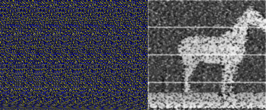
To do this project I created a small data set of “wall-eyed” random-dot autostereograms. There are other kinds of stereograms, that can be viewed in different ways, but I felt the random-dot ones would be slightly easier to decode. The basic premise is that for every small set of horizontal pixels there is a corresponding row of pixels some distance away. The distance between the matching rows segments is what your brain uses to get the depth map. The matching of the rows of pixels is periodic with a period related to the vergence distance you must view the image at. Figuring out the period of the image is easy, if you look at the image you can basically see columns of pixels. For most autostereograms there are usually between 6 and and 20 for a normal image, the horse image above has seven instances of the repeating patern. If you have an image that is 600 pixels wide, with about six columns, the pixel, or set of pixels at [0,0] will have a correspondence at roughly [100+d,0], where the value of d is the depth value.

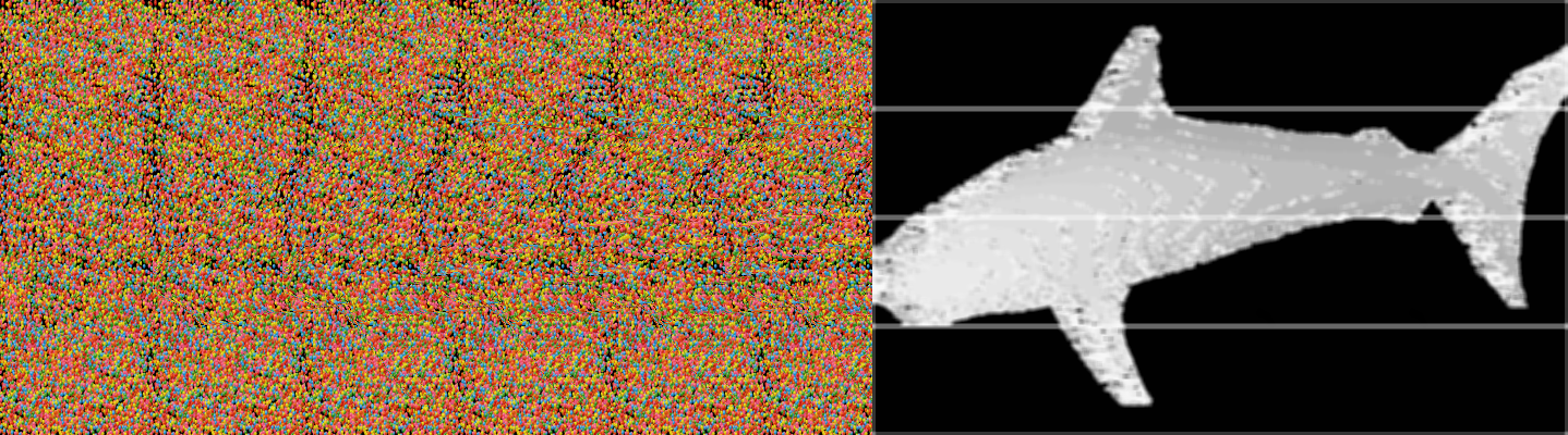
I baked up a naive algorithm in about 90 minutes and had an early prototype. The basic idea is that you iterate over the rows in the image, and for a small chunk of pixels in that row (roughly ten pixels) you search a window around where the correspondence should exist, and then record that value in a depth map. So for our example image 600 pixels wide, you would try to match pixels [0:10,0] with [100:110,0], [101:111,0] and so on until you found a decent match. For my first example I used the gray scale sum of absolute pixel differences. You could do a correlation, but I thought that the simple solution should suffice. It is worth noting that you can also move up to frequency space and do a multiplication of the spectra but that seemed like a lot of work. I googled a bit and found this example that does just that. That solution seems to get stronger edges, and work on a few different kinds of stereograms, but I would argue mine gets betters depth maps.
My first pass, using naive python looping worked but it was as slow as molasses in January. I decided to see if I could speed things up. The first speed hack I tried was to use an integral image. An integral image is an image where each pixel is the sum of the pixels above and to its left. Integral images are great if you want to calculate lots of different average values across an image really fast, and they are what makes Haar Cascades and face detection possible. In an integral image, once the integral is computed, the sum, and average of any area in the image can be computed with in just four look-ups, and three additions, which is a decent time savings. I modified my code and got maybe a 10-20% speed up (I didn’t bench mark it). Since the operations are done row-wise and each row is independent of the next one this algorithm is really well suited to parallelization. I decided to try my hand at doing some image processing using the python multiprocessing library. It took me about an hour to chunk out the code and get everything running, but it did improve performance significantly (a little less than 4x). I need to go back and refactor the code to deal with some bounds issues, which is causing the horizontal lines in the image, and perhaps use shared memory, but the results are well worth the effort. You can take a look at the code for yourself at this repo, I’ve put a gist of the code below for reference.
If I get some more time I want to see how much of a speed up Numba can get the naive implementation and possibly do some bench marking of the different approaches. I also need to remove the banding caused by the multiprocess “chunking.” The algorithms performance seems to be very dependent on the search window size so I would like to find a more robust way of determining the size of the search window, possibly by looking at low end of the FFT spectrum.